Welcome
-
-
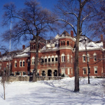
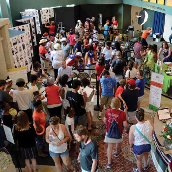
Greensboro and Triad History
-
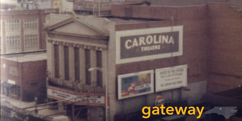
Collections from libraries, archives, and museums, as well as individuals, businesses, and community organizations throughout the area that document the history of Greensboro and the North Carolina Piedmont. Items include photographs, newspapers and magazines, personal and business records and papers, maps, city directories, and oral history interviews.
-
-
UNCG History
-
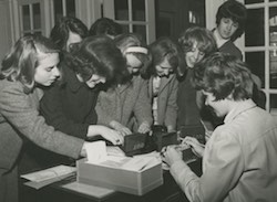
Collections from the Martha Blakeney Hodges Special Collections and University Archives that document the history of the university from its founding in 1892 as the State Normal and Industrial School to the present day. Items include photographs, university records, student and organizational scrapbooks, newspapers, yearbooks, course catalogs, and other materials.
-
-
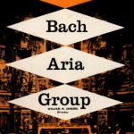
Visual and Performing Arts
-
Collections from the UNC Greensboro University Libraries and other sources that document the visual and performing arts. Items include a vast array of items from the cello collection at UNC Greensboro as well as playbills, photographs, scrapbooks, sheet music, and other mementos from a variety of sources at UNC Greensboro and the larger community.
-
-
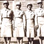
Women Veterans Historical Project
-
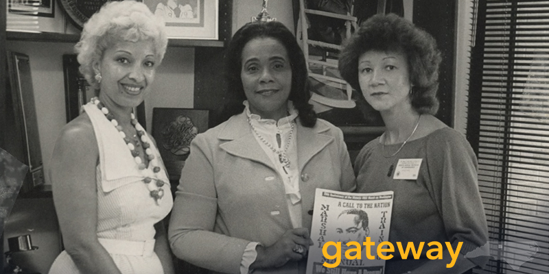
The Betty H. Carter Women Veterans Historical Project documents the contributions of women in the military and related service organizations since World War I. The project includes a wide range of source material including photographs, letters, diaries, scrapbooks, oral histories, military patches and insignia, uniforms, and posters, as well as published works.
-
-
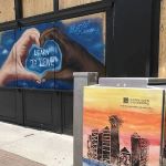
Highlights and Exhibits
-
Exhibits and other curated sets of items and collections focusing on specific themes relating to local history, social justice movements, and specific types of materials. These curated collections include items from multiple partners and are good "starting points" for exploring the material in Gateway. Many also include contextual materials and other study guides.
-
-
Partners and Collections
-
Libraries, museums, and archives around the Triad have collaborated with UNC Greensboro on digitization initiatives and Gateway is the host site for most of the material digitized in these collaborations. Explore our community partners and their individual contributions and also see links to additional content from our partners.
-
-
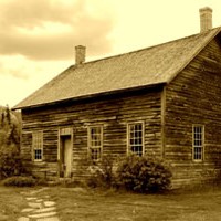
Digital Library on American Slavery
-
The Digital Library on American Slavery (DLAS) is an expanding resource compiling independent collections focused upon race and slavery in the American South, made searchable through a single, simple interface. DLAS incorporates all the material that was originally part of the North Carolina Runway Slave Ads project.